AI
Short-Term Memory Convolutions
Motivation
The successful deployment of a signal processing system necessitates the consideration of various factors. Among these factors, system latency plays significant role, as humans are highly sensitive to delays in perceived signals. In the context of audio-visual signals, individuals can detect delays between audio and visual stimuli exceeding 10 ms [1]. However, in conversational settings, the maximum acceptable latency can extend up to 40 ms [2, 3, 4]. To facilitate optimal human-device interactions in many audio applications, the buffer size is adjusted to align with the maximum acceptable latency.
When we process a continuous stream of incoming data using neural networks, it is referred to as online inference. This type of inference presents several challenges, including the minimization of latency and computational cost. For an online system to be considered real-time, the inference time must be shorter than the input length. To meet this requirement, one option is to increase the input length, but doing so would result in increased latency as we wait for the entire input. Conversely, reducing the input length leads to a higher number of calculations, as the network needs to be recalculated more frequently.
In this blog post, we describe a novel approach to data caching in convolutional layers known as Short-Term Memory Convolution (STMC). This approach enables the processing of arbitrary data chunks without incurring any computational overhead. Specifically, after model initialization, the computational cost of processing a chunk is linearly dependent on its size, thereby reducing overall computation time. Importantly, this method is applicable to various models and tasks, with the only prerequisite being the utilization of stacked convolutional layers.
Short-Term Memory Convolutions
To see STMC in practice, let’s assume the signal  and 2 convolutional kernels
  and
and  . When we apply those kernels to our input, we get:


The aggregate receptive field resulting from these two operations is equivalent to the sum of the kernel sizes. During inference, in order to obtain any output, the network requires an input of at least this size. However, providing the network with a direct input vector, denoted as  , matching its receptive field size introduces computational overhead. This is due to the fact that neural networks often have a larger receptive field compared to the quantity of data they receive. The visual representation depicted below illustrates this concept:

Figure 1. Convolution redundancy effect in time domain
To facilitate visualization, we have made the assumption that the receptive field of our network is 6 (assuming additional operations exist after the second convolution), and our kernels have a size of 2. In this particular example, there is an overlap observed between the inference at time step  and
and  . In practical terms, this implies that the calculations for the colored frames at time are unnecessary, as they were already computed at time . In order to fully reconstruct the output without incurring this computational overhead, we can store the outputs of each layer at every time step and pad the input of each convolutional/pooling layer to satisfy the layer-wise receptive fields. This process can be formulated as follows:

where  is Hadamard product,
  is data buffer, and
  is the operation done by shift register – data cropping and padding.
This method can be applied to various types of convolutions and poolings, including transposed convolutions. In our research, we have observed a natural anti-causality property associated with transposed convolutions. This anti-causality arises from the behavior of transposed convolutions, which add an additional frame to the right-most side of their output, where the most recent frames are located. This shifting of the output vector in time unfavorably affects causality, although it is important to note that the interpretation of the output vector also plays a significant role in determining causality. In order to implement the Short-Term Memory Convolution (STMC) approach for transposed convolutions, we first need to comprehend the arithmetic involved in their computations.
Let’s assume  and
and  as
as  input and
  output tensors and
  as convolutional layer with kernel. Transposed convolution can be then represented in a standard anti-causal way as follows:


The application of transposed convolutions involves performing standard convolutions with additional padding and data scattering. The size of the padding depends on the kernel size, while the size of scattering depends on the stride. To implement the transposed Short-Term Memory Convolution (tSTMC), we utilize this principle to create a fused operation that performs transposition in every axis except the time axis, where we apply the standard convolution. It is important to note that the standard convolution is utilized because the additional frames on the right-most part of the output are not required.
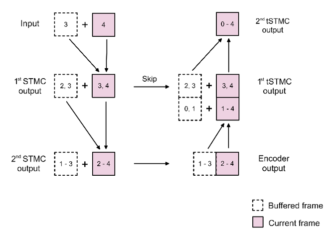
Figure 2. Exemplary depth-2 U-Net network with STMC/tSTMC
To summarize both proposed operations, please see the picture below.

Figure 3. A) Short-Term Memory Convolution B) Transposed Short-Term Memory Convolution
Experiments
The primary task we have chosen to showcase the benefits of the STMC/tSTMC scheme is speech separation. In this context, speech separation refers to the extraction of speech signals from background interference, encompassing various sources of noise. For the purpose of obtaining a clean speech signal, the task can be interpreted as speech denoising or noise suppression. To maintain clarity, we will refer to this task as speech separation.
As our baseline model, we have employed a network based on the U-Net architecture [5]. However, we have simplified the original architecture by removing max pooling operations, resulting in encoding being solely performed by convolutions. We have adapted this model specifically for the audio separation task and achieved satisfactory results with a model depth of 7. Each convolutional layer comprises multiple kernels with a length of 3 in the time domain, leading to a receptive field of 29 for the assembled network. The kernel size in the frequency domain is set to 5.
Since the benchmark network consists of convolutional layers that are locally centered [6] around the current time frame, we can derive a receptive field of 14 for both the past and future context. The input to the network utilizes the Short-Time Fourier Transform (STFT), with separate channels for the real and imaginary parts, resulting in a complex mask as the network's output for the input signal. A STFT window of size 1024 and a hop size of 256 are employed.
The results for all tested models are presented side-by-side in Table 1. Comparing to standard convolutions, the incremental inference (INC) method [7] achieves an 8.00-fold and a 29.74-fold latency reduction in the case of non-causal and causal setting, respectively. Our method (STMC) outperforms INC with a further 1.32-fold latency reduction for non-casual and a 2.52-fold reduction for causal variants.
STMC achieved also approximately 5.68-fold reduction in inference time, compared to INC. The impact of STMC on the non-causal U-Net is lower as most of the computational cost of U-Net STMC is due to the need for waiting for the future context (convolutional kernels centered with respect to the output). The implementation of transposed STMC in the decoder of the Causal U-Net model gives only a slight improvement in latency (0.57 ms), but it reduces the peak memory consumption by approximately 20%. The model size is similar for standard, INC, and STMC variants. The causal models are approximately 33% smaller than the non-causal ones, which is caused by the smaller kernels which look only in the past direction.
In the tested models, the incremental inference (INC) method [7] demonstrates a significant reduction in latency. Specifically, compared to standard convolutions, INC achieves an 8.00-fold reduction in latency for the non-causal setting and a 29.74-fold reduction for the causal setting. Our proposed method, Short-Term Memory Convolution (STMC), surpasses INC by providing an additional 1.32-fold reduction in latency for the non-causal variant and a 2.52-fold reduction for the causal variant. Furthermore, STMC achieves an approximate 5.68-fold reduction in overall inference time compared to INC.
It is important to note that the impact of STMC on the non-causal U-Net model is relatively lower. This is primarily because the majority of the inference time of U-Net STMC is attributed to waiting for the future context (convolutional kernels centered with respect to the output). On the other hand, incorporating transposed STMC in the decoder of the Causal U-Net model results in only a slight improvement in latency (0.57 ms), but it significantly reduces peak memory consumption by approximately 20%.
In terms of model size, the standard, INC, and STMC variants have similar sizes. However, the causal models are approximately 33% smaller than the non-causal ones. This reduction in size is a result of the smaller kernels used in the causal models, which only consider the past direction.
Table 1. Results of evaluation on desktop using TFLite Model Benchmark Tool. ’C.’ stands for causal
* Difference in metrics due to separate learning of models.
The results depicted by fig. 4 provide insights into how STMC performs with models of different sizes. The SI-SNRi metric remains the same for both INC and STMC models. The absolute peak memory consumption improvement achieved by STMC scales linearly with model size, while the relative improvement compared to INC linearly decreases from 16% to 11%.
In terms of inference time, STMC has a significant impact on all tested models, and the inference time scales linearly with model size. The speed-up of STMC over INC for this particular architecture remains constant at around 81%, except for models of size 1.32 MB and smaller, where the speed-up drops to approximately 74%.

Figure 4. Influence of model size on STMC. A) SI-SNRi B) Improvement over peak memory consumption C) Inference time D) STMC speed-up over INC
The last conducted experiment measured the SI-SNRi metrics of models using different lengths of look-ahead. The results, as shown in Figure 5, indicate that increasing the look-ahead length has a positive impact on the metrics.
It is important to note that the experiment confirms a 6% decrease in metrics, which is solely attributed to the lack of future content. In this test, an interpolation between causal and non-causal networks from the main experiment was performed. The determined characteristic is non-linear, with the first frames appearing to have a more significant impact compared to the future frames on the right side of the plot. Specifically, the first frame increases SI-SNRi by 0.177 dB, while the last frame increases it by 0.019 dB.
To provide a comprehensive analysis, error bars have been included in the plot. These error bars represent the significant differences observed between the same models in this particular experiment. Each specific look-ahead length includes all SI-SNRi results on the validation dataset achieved by the five models trained for that specific look-ahead length.

Figure 5. Influence of look-ahead on SI-SNRi
Conclusion
In this blog post, we have described a method to address several important aspects of convolutional neural network (CNN) models, including inference time, latency, memory consumption, and computational complexity. The proposed method is based on buffering past states of the model at each convolutional and pooling layer, allowing for the efficient reconstruction of the model's receptive field. Importantly, this method does not compromise the output quality of the model.
By leveraging the STMC method, we can achieve improved efficiency and resource utilization in CNN models without sacrificing the quality of their outputs. This has important implications for a wide range of applications that rely on CNNs, enabling more efficient and effective deployment in real-world scenarios.
Link to the paper
https://arxiv.org/abs/2302.04331References
[1] Andrew Mcpherson, Robert Jack, and Giulio Moro. Action-sound latency: Are our tools fast enough? In The International Conference on New Interfaces for Musical Expression, April 2016.
[2] Alberta Ipser, Vlera Agolli, Anisa Bajraktari, Fatimah Al-Alawi, Nurfitriani Djaafara, and Elliot D. Freeman. Sight and sound persistently out of synch: stable individual differences in audiovisual synchronisation revealed by implicit measures of lip-voice integration. Scientific Reports, 7(1):46413, April 2017. ISSN 2045-2322.
[3] Philip Jaekl, Jakob Seidlitz, Laurence R. Harris, and Duje Tadin. Audiovisual delay as a novel cue to visual distance. PLOS ONE, 10(10):1–12, October 2015
[4] Nicolas Staelens, Jonas De Meulenaere, Lizzy Bleumers, Glenn Van Wallendael, Jan De Cock, Koen Geeraert, Nick Vercammen, Wendy Van den Broeck, Brecht Vermeulen, Rik Van de Walle, and Piet Demeester. Assessing the importance of audio/video synchro-nization for simultaneous translation of video sequences. Multimedia Systems, 18(6):445–457, November 2012. ISSN 1432-1882.
[5] Olaf Ronneberger, Philipp Fischer, and Thomas Brox. U-net: Convolutional networks for biomedical image segmentation. In MICCAI, 2015.
[6] Alessandro Favero, Francesco Cagnetta, and Matthieu Wyart. Locality defeats the curse of dimensionality in convolutional teacher-student scenarios. In Advances in Neural Information Processing Systems, 2021
[7] Michal Romaniuk, Piotr Masztalski, Karol Piaskowski, and Mateusz Matuszewski. Efficient Low-Latency Speech Enhancement with Mobile Audio Streaming Networks. In Proc. Interspeech 2020, pp. 3296–3300, 2020.