Introduction

Figure 1. Visual representation of DSS with background noise

Distance-based source separation (DSS) is a recently developed approach to audio separation that classifies sources as “near” or “far” based on their distance from a reference microphone. Unlike traditional source separation, DSS leverages spatial cues—such as the inverse-square law for sound intensity, direct-to-reverberation ratio (DRR), and other distance-related acoustic effects—to separate a mixed audio signal into components by distance. For example, in a conference room or lecture hall, a DSS system can isolate the speech of a nearby presenter from other voices further away by recognizing distance-induced differences in audio characteristics.

Until now, research on DSS has focused exclusively on indoor environments. Existing methods [1-3] assumed controlled indoor acoustics, and they struggle when applied to outdoor scenarios. Outdoor environments introduce new challenges: wind and ambient noise, lack of clear reverberant boundaries, and unpredictable acoustic conditions can all degrade the performance of models trained only on indoor data. In high-noise outdoor settings, even measuring DRR reliably is difficult, making it hard for a model to distinguish a distant speaker from background noise. Thus, there has been a pressing need to extend DSS to noisy outdoor conditions.

Another practical demand is to enable DSS on mobile devices. Many users record videos on smartphones and wish to enhance the audio by isolating a speaker’s voice from environmental noise. This requires a DSS model that is not only accurate in varied environments but also efficient enough for real-time execution on mobile hardware. Prior DSS studies did not address on-device performance, leaving a gap between research prototypes and deployable solutions.

Our work is the first to tackle DSS in noisy outdoor environments and on mobile devices. We present a novel single-channel DSS model that operates robustly in both outdoor and indoor scenarios. Key innovations include a two-stage Conformer architecture for capturing complex audio dependencies, a linear relation-aware self-attention (RSA) mechanism for efficiency, and optimizations for mobile GPU acceleration using the TensorFlow Lite (TFLite) GPU delegate. The result is a model that achieves effective near/far voice separation even in windy outdoor conditions, while running in real time on a smartphone with vastly improved energy efficiency. In the following sections, we describe the model’s architecture and optimizations, the simulation of outdoor acoustic conditions for training, and our benchmark results demonstrating superior performance in both accuracy and on-device speed.

Proposed Architecture

Figure 2. Schematic diagrams of MBaseline architecture

Two-Stage Conformer Blocks for DSS: Our DSS model builds upon a Conformer-based encoder-decoder separation framework inspired by CMGAN [9], a state-of-the-art speech enhancement architecture. The baseline architecture (named MBaseline) uses four repeated two-stage Conformer (TS-Conformer) blocks as the separator. Each TS-Conformer block is a variant of the Conformer layer designed to capture both time-domain and frequency-domain dependencies. It combines multi-head self-attention (for global context across the time sequence) with convolutional layers (for local feature extraction), which is ideal for modeling speech signals that have structure in both time and frequency. In our two-stage design, each block operates in a dual-path manner: one stage processes frames within a local chunk, and a second stage processes the sequence of chunks (similar in spirit to dual-path RNN separation networks). This hierarchy enables the model to handle long audio sequences efficiently while still focusing on fine-grained temporal details.

The overall architecture is an encoder-separator-decoder pipeline. The encoder first transforms the input waveform into a compressed complex spectrogram representation using STFT and a learned compression (as in CMGAN). The separator then applies the four TS-Conformer blocks sequentially to this encoded representation. Notably, after the 2nd and 4th TS-Conformer blocks, the model branches into two outputs: one targeting the “near” source and one for the “far” source. Two parallel decoders – a Mask Decoder and a Complex Decoder – reconstruct the waveform for each target. The Mask Decoder produces a spectral mask to extract the target magnitude, while the Complex Decoder predicts the real and imaginary components to refine phase information. The final separated signals are obtained by multiplying the input spectrogram by the mask and adding the predicted complex spectrogram, then applying an inverse STFT to get time-domain audio. By using two dedicated decoders, the model can separately optimize for near and far source reconstruction. This architecture proved effective at isolating a close speaker’s voice (near output) versus distant background speech/noise (far output) from a single-channel mixture.

Linear Relation-Aware Self-Attention (RSA): The Conformer’s multi-head self-attention mechanism originally included RSA [16], which incorporates relative positional encodings to better capture sequence order relationships. Standard RSA computes attention with a quadratic complexity O(N^2) in the sequence length N, which becomes a bottleneck for long audio. To overcome this, we replaced the standard RSA with a linear-complexity RSA. Our linear RSA is inspired by recent linear attention techniques, in particular Efficient Attention [5] mechanisms and Rotary Position Embeddings (RoPE) [6] as used in LinearSpeech [20]. The key idea is to avoid explicitly computing the full N x N attention matrix. We map queries and keys into a higher-dimensional feature space using kernel functions (here we use the softmax function as the feature map) such that dot-products in that space approximate the attention outcome. We also apply RoPE to encode relative positions without large trainable matrices. The resulting attention computation scales as O(N*d^2) (with d the feature dimension) instead of O(N^2 * d), dramatically improving efficiency for long sequences. While a quadratic RSA might capture fine-grained physical cues slightly better, our experiments showed that linear RSA actually improved the model’s context awareness and yielded equal or better separation performance – likely because it enables using longer context windows with the same computation budget. Crucially, linear RSA reduces memory usage and speeds up inference, which is important for mobile deployment.

Mobile GPU Optimization: To run the model on a smartphone in real time, we optimized it for the TensorFlow Lite GPU delegate. Mobile GPUs excel at parallel float32/float16 operations and can vastly accelerate neural network inference. However, not all TensorFlow operations are supported by the TFLite GPU delegate, and certain patterns (like dynamic tensor shapes) can force fallback to CPU. We followed two rules: (1) use only GPU-supported layers, and (2) keep tensor shapes (batch and dimensions) consistent throughout the network. In practice, this meant making a few careful modifications. For example, we removed any tensor reshaping inside the TS-Conformer blocks that would alter batch dimensions. Instead of using the built-in 1-D convolution that internally reshapes data, we implemented a custom 1-D convolution layer that preserves the batch dimension, thereby avoiding unsupported ops. We also fixed the batch size to a constant (4 in our experiments) and ensured all intermediate tensors explicitly maintain this batch size to prevent runtime shape mismatches. Additionally, we adjusted the multi-head attention computation to split the operation across the feature axis (h-axis) so it could be handled as separate batch operations, because the default implementation of batch matrix multiply was not fully supported on GPU. By disabling certain minor TensorFlow optimizations (e.g. we turned off the “unfold batch matmul” option), we allowed the GPU delegate to execute the attention as intended. After these changes, our entire model (dubbed MProposed) runs using the TFLite GPU delegate with no CPU fallback – meaning the phone’s GPU handles 100% of the operations. This enables substantial speed-ups and energy savings, as detailed below.

Simulation of Outdoor and Indoor Audio Environments

To train and evaluate the model, we needed data representing diverse acoustic environments. Real recordings with ground-truth “near” and “far” source separation are scarce, so we built a large simulated dataset using a combination of clean speech corpora and acoustic room simulation. We leveraged the Pyroomacoustics [7] toolbox to generate realistic room impulse responses via the Image Source Method (ISM) [8]. The simulation parameters were randomized to cover a wide range of scenarios:

Room geometry: For “indoor” simulations, room dimensions were sampled around 6m × 6m × 2.6m (with random variation). For “outdoor” simulations, we approximated an open space by setting the walls (except the floor) to be anechoic (no reflections), effectively simulating only direct paths and a ground reflection.

Microphone and source placement: The microphone was placed roughly at the room center (randomly within ~0.3m of center). For each mixture, we placed one or more speech sources in the room – some near the mic, others far. Near-source distances were sampled between 0.02 m (practically at the mic) and 0.5 m, while far sources were placed between 1.3 m and 1.7 m away. We set 0.5 m as the distance threshold to classify near vs. far. Any source beyond 1.7 m was considered an unseen far region during training, which allowed us to test the model’s generalization to even greater distances.

Reverberation and noise: We varied the reverberation time (RT60) from 0.15 s up to 1.0 s to include both damped and very echoey environments. After convolving source signals with the simulated room impulse responses, we added background noise at random signal-to-noise ratios (SNR) of 0, 5, 10, 15, or 20 dB. The noise clips were drawn from a large collection of real-world recordings (e.g. crowd chatter, wind, traffic, etc.), ensuring the mixtures include challenging ambient noise typical of outdoors.

Using this procedure, we used the CSTR-VCTK [23], AISHELL-3 [24], and AI-Hub datasets[25-27] to generate a massive training dataset resampled at 16 kHz. The dataset contains approximately 5,000 hours of speech data, including about 500 speakers, 5 languages, and 8 emotion styles. It also contains approximately 1,000 hours of sound data from noisy environments, classified into various categories. Each training example is a 3-second mixture constructed by randomly selecting 1–3 near speakers and 1–3 far speakers and mixing their processed signals (plus noise). For evaluation, we similarly created simulated test sets: 100 samples for indoor and 200 samples for outdoor conditions, using held-out speech from WSJ0 corpus and a separate 30-hour noise dataset not seen in training.

One important question was how much outdoor data to include in training. We experimented with different indoor:outdoor mixing ratios. The outcome was that a mix of 60% indoor + 40% outdoor examples in training gave the best overall performance, outperforming 100% indoor (which lacked outdoor diversity) as well as extreme fine-tuning strategies. Therefore, our final model was trained on a balanced mix, which did not sacrifice indoor performance but significantly boosted outdoor robustness (as shown next).

Experiments and Results

1. Separation Performance

We evaluated the source separation quality using scale-invariant signal-to-distortion ratio improvement (SI-SDRi) [30]. This metric measures how much the model improves the clarity of target signals (near or far) relative to the input mixture. We compared several model variants:

Table 1. Test results of all architectures for indoor test datasets. Each cell represents the average SI-SDRi (dB) of (near / far)

On indoor test mixtures, the proposed model achieved the best SI-SDR improvements for both near and far sources. For example, in cases with one near and one far speaker, MProposed achieved 5.5 dB (near) / 12.0 dB (far) SI-SDRi, versus 5.3/11.5 dB for MBaseline. This indicates that replacing RSA with our linear version did not degrade performance; in fact, it slightly improved it. We also observed the importance of the Conformer-based (MRoformer) underperformed (e.g., only 3.9/9.7 dB in that scenario), showing the Conformer’s convolutional modules add value for DSS. The DPRNN model (MTF-DPRNN) had strong near-source results in multi-speaker scenarios (it excelled at extracting a speech source and treating everything else as noise), but it struggled in cases where only one class of source was present. For instance, if the mixture had only a far speaker (and noise), DPRNN sometimes mistakenly pulled out speech where there was none, or vice versa. This is likely because DPRNN specialized in separating speech from noise, rather than two speech streams by distance. Our Conformer approach, on the other hand, consistently handled both near and far outputs.

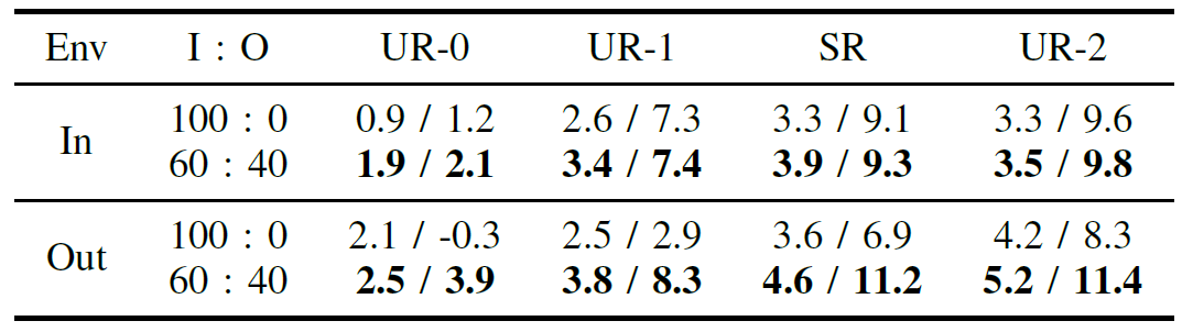
Table 2. Test results of two MProposed using the datasets mixed in 100% indoor and 60:40 indoor/outdoor, respectively. Each cell represents the average SI-SDRi (dB) of (near / far).

We then tested on more challenging outdoor mixtures. Here the benefit of training with outdoor data became evident. An MProposed model trained on 100% indoor data saw a severe drop in far-source performance in windy or noisy outdoor conditions (sometimes even yielding negative SI-SDRi, meaning it made the distant speech worse by amplifying noise). In contrast, the same model trained with 60:40 indoor/outdoor data maintained high performance outdoors, clearly separating distant speech from noise. For example, on a windy outdoor recording of two men speaking (one near, one far from the mic), the indoor-trained model (achieved far SI-SDRi of -0.3 dB) essentially failed to separate the far speech from wind noise. Our proposed model with outdoor training (achieved +3.9 dB far SI-SDRi) clearly separated in the same scenario – a substantial improvement, turning an unusable output into a clearly intelligible distant voice. Across various distances, we found that including outdoor data improved far-source separation by 3–5 dB on average in outdoor tests, while also slightly boosting near-source performance. Importantly, these gains did not come at the expense of indoor performance: the mixed-trained model was equal or better on indoor tests compared to the indoor-only model. This suggests that the model effectively learns generalizable features for distance that apply to both environments, and the outdoor noise exposure simply makes it more robust.

Figure 3. Results for a real outdoor sample

Figure 3 depicts spectrogram outputs of the MProposed model on a real 5-second outdoor recording with a near and a far speaker talking amid wind noise. The top row shows the separated near (left) and far (right) spectrograms when the model is trained on a mix of indoor+outdoor data (60:40 ratio). The bottom row shows the outputs of the same model architecture trained on indoor data only (100:0). In the top far spectrogram, the distant speech (upper frequencies with voiced harmonics) is clearly separated from the wind noise (low-frequency background), whereas in the bottom far spectrogram, the model trained without outdoor data fails to distinguish the far speech from noise (resulting in a nearly blank output). This visualizes the advantage of including outdoor scenarios in training – the model can recover the distant speaker’s voice even under strong wind interference.

2. On-Device Benchmarking

We deployed our models on a Samsung Galaxy S23 smartphone to measure real-world mobile performance. We evaluated two key aspects: inference speed (Real-Time Factor, RTF) and energy consumption. RTF is defined such that 1.0 means processing one second of audio takes one second of runtime (so lower is faster). An RTF < 1 is required for real-time processing. We used a 5-minute sample audio (split into 3-second chunks) for each test and measured average CPU/GPU usage and power draw (using Android’s dumpsys tool [21]).

Table 3. Mobile benchmark performances of all architectures

Table 3 shows on-device efficiency comparison on a Galaxy S23 (TFLite). Energy % is the proportion of battery used per minute (lower is better). RTF less than 1 indicates faster than real-time processing. MBaseline and MTF-DPRNN could not fully run on the GPU (due to unsupported layers as noted earlier), so their GPU entries are blank – they ran on CPU only. Our MProposed model, however, ran entirely on the GPU, achieving an RTF of 0.16, meaning it can process audio about 6× faster than real time on the phone. This is a 10× speed-up over the 1.55 RTF on CPU. In other words, a 3-second clip takes ~0.48 s to process on GPU vs ~4.65 s on CPU. The energy savings are even more dramatic: the CPU version consumed ~3% of battery per minute of continuous processing, whereas the GPU version used only 0.15% per minute. This is a 20× reduction in energy, which is critical for mobile use (prolonged recording and processing would drain a battery quickly on CPU). These measurements validate that our GPU-focused design successfully delivers real-time performance on device. The efficient linear RSA and lightweight TS-Conformer design keep the model small (1.3M parameters) and computationally manageable (25.7 GMac/s), so it fits the constraints of mobile inference.

For reference, the table also shows the “encoder+decoder only” model (MEnc&Dec), which is extremely fast (0.10 RTF on GPU) but has no separation capability, and thus low computational load. Our full model is only slightly heavier, demonstrating the optimization success. Compared to MTF-DPRNN, which had a similar parameter count, MProposed on GPU is far superior in speed since MTF-DPRNN cannot leverage the GPU at all. In summary, MProposed is the only model among those tested that achieves real-time separation on the mobile GPU with negligible battery impact, making it highly practical for on-device applications.

Conclusions

We have introduced a new single-channel DSS system that extends audio source separation to challenging outdoor environments for the first time. By leveraging a two-stage Conformer architecture and a linearized self-attention mechanism, our model can discern between nearby and distant sound sources using subtle acoustic cues, even in the presence of wind or crowd noise. We further demonstrated how careful co-design of the model with mobile hardware constraints (using TFLite GPU delegation) enables real-time performance on a Galaxy smartphone with an order-of-magnitude reduction in energy consumption. In both outdoor and indoor tests, the proposed model trained with a mix of outdoor data outperformed a model trained on indoor data alone, highlighting the importance of diverse training for robust DSS.

This research opens up new possibilities for on-device audio enhancement: for example, smartphone users recording video in a noisy street could automatically isolate their own voice (near source) from the background chatter (far sources). To our knowledge, this is the first study to successfully achieve distance-based source separation in such on-device, in-the-wild conditions. Future work may explore addressing the residual challenges (we observed, for instance, that when a “near” speaker is extremely close to the threshold distance, the model can occasionally confuse it with “far” due to ambiguous cues [31]). Integrating additional information such as learned distance embeddings or multi-microphone data could further improve robustness in edge cases. Nonetheless, our current results demonstrate a significant step toward intelligent audio processing that adapts to the listener’s context – bringing clear voice separation to both the boardroom and the outdoors, right from your pocket.

Audio samples can be found online (https://icassp2025-hanbin-bae.netlify.app).
* This study used datasets from ‘The Open AI Dataset Project (AI-Hub, South Korea)’. All data information can be accessed through ‘AI-Hub (www.aihub.or.kr)’

Link to the paper

https://ieeexplore.ieee.org/abstract/document/10889318

View More

Close

References

[1] K. Patterson, K. Wilson, S. Wisdom, and J. R. Hershey, “Distance-Based Sound Separation,” in Proc. Interspeech, 2022, pp. 901–905.
[2] J. Lin et al., “Focus on the Sound around You: Monaural Target Speaker Extraction via Distance and Speaker Information,” in Proc. Interspeech, 2023, pp. 2488–2492.
[3] D. Petermann and M. Kim, “Hyperbolic distance-based speech separation,” in Proc. ICASSP, 2024.
[4] S. Kuznetsov and E. Paulos, “Rise of the expert amateur: DIY projects, communities, and cultures,” in Proc. Nordic CHI, 2010, pp. 295–304.
[5] Z. Shen et al., “Efficient Attention: Attention with Linear Complexities,” in Proc. WACV, 2021, pp. 3531–3539.
[6] J. Su et al., “RoFormer: Enhanced transformer with rotary position embedding,” Neurocomputing, vol. 568, 2024, Art. no. 127063.
[7] R. Scheibler, E. Bezzam, and I. Dokmanic, “Pyroomacoustics: A Python package for audio room simulation and array processing,” in Proc. ICASSP, 2018, pp. 351–355.
[8] J. B. Allen and D. A. Berkley, “Image method for efficiently simulating small-room acoustics,” J. Acoust. Soc. Am., vol. 65, no. 4, pp. 943–950, 1979.
[9] R. Cao, S. Abdulatif, and B. Yang, “CMGAN: Conformer-based Metric GAN for speech enhancement,” in Proc. Interspeech, 2022, pp. 4267–4271.
[10] A. Gulati et al., “Conformer: Convolution-augmented transformer for speech recognition,” in Proc. Interspeech, 2020, pp. 5036–5040.
[11] S.-W. Fu et al., “MetricGAN: Generative adversarial networks based black-box metric scores optimization for speech enhancement,” in Proc. ICML, 2019, pp. 2031–2041.
[12] S. Braun and I. J. Tashev, “A consolidated view of loss functions for deep learning-based speech enhancement,” in Proc. TSP, 2021, pp. 72–76.
[13] A. Pandey and D. Wang, “Densely connected neural network with dilated convolutions for real-time speech enhancement in the time domain,” in Proc. ICASSP, 2020, pp. 6629–6633.
[14] A. Vaswani et al., “Attention is all you need,” in Proc. NeurIPS, 2017, vol. 30, pp. 5998–6008.
[15] S. Chen et al., “Continuous speech separation with Conformer,” in Proc. ICASSP, 2021, pp. 5749–5753.
[16] P. Shaw, J. Uszkoreit, and A. Vaswani, “Self-attention with relative position representations,” in Proc. NAACL-HLT, 2018, pp. 464–468.
[17] R. Child et al., “Generating long sequences with sparse transformers,” arXiv:1904.10509, 2019.
[18] K. Yue et al., “Compact generalized non-local network,” in Proc. NeurIPS, 2018, pp. 6511–6520.
[19] S. Zhang, S. Yan, and X. He, “LatentGNN: Learning efficient non-local relations for visual recognition,” in Proc. ICML, 2019, pp. 7374–7383.
[20] H. Zhang et al., “LinearSpeech: Parallel text-to-speech with linear complexity,” in Proc. Interspeech, 2021, pp. 4129–4133.
[21] Android Developers, “Android studio dumpsys toolbox,” Online: developer.android.com/tools/dumpsys (accessed Feb. 29, 2024).
[22] Y. Luo, Z. Chen, and T. Yoshioka, “Dual-path RNN: Efficient long sequence modeling for time-domain single-channel speech separation,” in Proc. ICASSP, 2020, pp. 46–50.
[23] J. Yamagishi, C. Veaux, and K. MacDonald, “CSTR VCTK Corpus: English multi-speaker corpus for CSTR voice cloning toolkit (version 0.92),” 2017.
[24] Y. Shi et al., “AISHELL-3: A multi-speaker mandarin TTS corpus and the baselines,” 2020.
[25] Korea AI Hub, “Various emotion and intonation dataset for speech synthesis,” Online: aihub.or.kr (accessed Feb. 29, 2024).
[26] Korea AI Hub, “Neutral style multi-lingual translation dataset,” Online: aihub.or.kr (accessed Feb. 29, 2024).
[27] Korea AI Hub, “Extreme noise environment sound dataset,” Online: aihub.or.kr (accessed Feb. 29, 2024).
[28] J. S. Garofolo et al., “CSR-I (WSJ0) complete,” LDC, 2007.
[29] I. Loshchilov and F. Hutter, “Decoupled weight decay regularization,” in Proc. ICLR, 2019.
[30] J. Le Roux, S. Wisdom, H. Erdogan, and J. R. Hershey, “SDR – half-baked or well done?” in Proc. ICASSP, 2018, pp. 626–630.
[31] X. Liu and J. Pons, “On permutation invariant training for speech source separation,” in Proc. ICASSP, 2021, pp. 3425–3429.