AI
[CVPR 2022 Series #6] Gaussian Process Modeling of Approximate Inference Errors for Variational Autoencoders
|
The Computer Vision and Pattern Recognition Conference (CVPR) is a world-renowned international Artificial Intelligence (AI) conference co-hosted by the Institute of Electrical and Electronics Engineers (IEEE) and the Computer Vision Foundation (CVF) which has been running since 1983. CVPR is widely considered to be one of the three most significant international conferences in the field of computer vision, alongside the International Conference on Computer Vision (ICCV) and the European Conference on Computer Vision (ECCV). This year Samsung Research’s R&D centers around the world present a total of 20 thesis papers at the CVPR 2022. In this relay series, we are introducing a summary of the 6 research papers. Here is a summary of the 6 research papers among 20 thesis papers shared at CVPR 2022. - Part 1 : Probabilistic Procedure Planning in Instructional Videos (by Samsung AI Center – Toronto) - Part 3 : GP2: A Training Scheme for 3D Geometry-Preserving and General-Purpose Depth Estimation - Part 4 : Stereo Magnification with Multi-Layer Images(by Samsung AI Center - Moscow) - Part 5 : P>M>F: The Pre-Training, Meta-Training and Fine-Tuning Pipeline for Few-Shot Learning - Part 6 : Gaussian Process Modeling of Approximate Inference Errors for Variational Autoencoders |
About Samsung AI Center – Cambridge
Many technical challenges must be overcome to provide excellent AI experience to users of Samsung devices. The Cambridge AI Center focuses on 'multimodal AI' technology, 'data efficient AI' and 'On-device AI technology that makes AI models work efficiently and robustly on Samsung's devices'.
First, it is essential to handle multimodality for a natural interaction experience with users. Second, AI model needs to be updated from less learning data to provide users with customized services and experiences. Lastly, these experiences should be able to achieve optimal performance for each device in various specs, and at the same time users expect the AI model to be consistently good even in a wide variety of daily environments.
In this year’s CVPR, Cambridge AI Center has published papers related to the acceleration of the inference process of VAE and the technology that improve the accuracy of the few-shot learning. In these papers, researchers propose new ideas in terms of 'deploying an efficient AI model for Samsung devices' and 'increasing the accuracy of the AI model in a user environment where there’s a few label data.'
Through future research, we will continue to develop technologies that innovate the efficiency and usability of the AI model for Samsung devices and services.
Introduction
Variational Autoencoder (VAE) [5,6] is one of the most popular deep latent variable models in modern machine learning. In VAE, we have a rich representational capacity to model a complex generative process of synthesizing images (x) from the latent variables (z). And at the same time it provides us with the interpretability of how a given image x is synthesized, namely the probabilistic inference (inferring the most probable latent state z that produced x).
The central component of VAE is the amortized inference, which replaces the instance-wise variational inference optimization with a single neural network feed-forward pass, thus allowing fast inference. However, this comes at the cost of accuracy degradation, known as the amortization error.
Several recent approaches aimed to reduce the amortization error while retaining the computational speed-up from amortized inference. Our earlier work of Recursive Mixture Inference [1] (See also our earlier blog post https://research.samsung.com/blog/Fast-and-Accurate-Inference-in-Variational-Autoencoders.) was one successful attempt, and in the current blog we will propose another approach.
Our key insight is to view the amortization error in VAE as random noise, and we model it with a stochastic random process (specifically, the Gaussian process [2]). The main advantage of this stochastic treatment is uncertainty quantification: we can quantify how uncertain or difficult it is to approximate the posterior distribution by neural network amortization.
We not only reduce the amortization error by marginalizing out the noise, but we can also measure instance-wise difficulty in amortized inference approximation (e.g., amortized inference is more accurate for some instances than others).
VAE and Amortized Inference
This section provides a very brief overview of VAE and amortized inference. For more detailed descriptions, we refer the readers to our earlier blog post https://research.samsung.com/blog/Fast-and-Accurate-Inference-in-Variational-Autoencoders.
VAE’s generative process is composed of a prior (e.g., standard normal) on the latent variables and the conditional decoding process, where the latter is modeled by a (deep) neural network with parameters 

The inference with a given  amounts to evaluating the posterior distribution
  , which is unfortunately infeasible due to the intractable normalizing constant. The (stochastic) variational inference (SVI) aims to approximate the posterior by a tractable distribution such as Gaussian
  , whose parameters
  are determined by the following optimization:

It can be shown that the KL divergence equals (up to constant) the so-called ELBO (evidence lower bound) function  with the opposite sign,

Then, the KL minimization is equivalent to ELBO maximization, which can be tractably done by stochastic gradient descent (SGD). However, the critical drawback is that the ELBO objective is specific to each instance x, and when a new instance x comes in, the SGD optimization has to be performed from the outset. That is, SVI is computationally very expensive.
SVI’s computational issue can be addressed by the amortized inference (AVI) [5,6]. The optimal solution of the SVI optimization problem can be seen as a function of  , i.e.,
  , and we can train a neural network to mimic this function
  (Figure. 1). With AVI, the inference is done by a single feed-forward pass through a neural network instead of the time-consuming instance-wise SVI optimization. However, this computational advantage comes with a cost; AVI is fast, but less accurate than SVI due to the neural net function approximation error, known as the amortization gap (Figure. 2).
Although there were some hybrid approaches called semi-amortized VI (SAVI) [7], which initialize the encoder by AVI and take a few SGD steps afterwards to reduce the amortization error. But, SAVI still suffers from computational overhead due to the extra SGD steps and high-order derivatives.

Figure 1. Amortized inference. It replaces the SVI optimization problem by a single feed-forward pass through a neural network called the inference/encoder network  with parameters
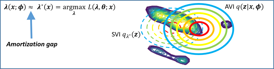
Figure 2. Amortization gap makes AVI less accurate than SVI
Our Approach: Gaussian Process Error Modeling
Our main idea is to view the amortization error as random noise, and model it with a stochastic process such as the Gaussian process. The Gaussian process (GP) is an extension of a Gaussian-distributed random vector to a distribution over functions, where the covariance of the distribution is specified by a kernel function  That is, for any set of points
  , the vector
  is distributed by Gaussian
  where
where ![]() is the
is the  covariance matrix
We write the means and standard deviations of the amortized posterior  as functions, and decompose them into: the AVI prediction (mean
  and standard deviation
  ), and the error terms
  and
and  as follows:

For instance,  and
and  amount to the difference in mean and standard deviation between SVI’s
  and
and  in Figure. 2. We let these error functions
  and
and  be distributed as GP a priori,
  To link this prior belief to the actual outcome/observation
  we define the likelihood function as the VAE’s ELBO function (a lower bound of

Then given the training data  , we have the posterior distribution for the errors and .

For tractable GP posterior inference, we adopt the linear deep kernel trick [3], essentially writing the GP functions as feature times weights product forms,

This allows a weight space posterior derivation,

The posterior is approximated by a Gaussian  with variational inference, i.e., minimizing the following objective:

Experimental Results
To see the improvement in the posterior approximation accuracy, we measure the generalization performance, specifically the test log-likelihood scores, on several benchmark datasets.
Please refer to our paper [1] for full experimental details. Our approach (dubbed GPVAE) is contrasted with the vanilla VAE (AVI), SAVI [7], the flow-based model IAF [8] that has rich representational capacity, and our earlier mixture-based inference [4]. The results are summarized in Table 1. Compared to these competing methods, our GPVAE performs the best throughout all datasets with strong statistical significance. Furthermore, when it comes to the test inference time, our approach is faster than SAVI, while being comparable to flow-based models.
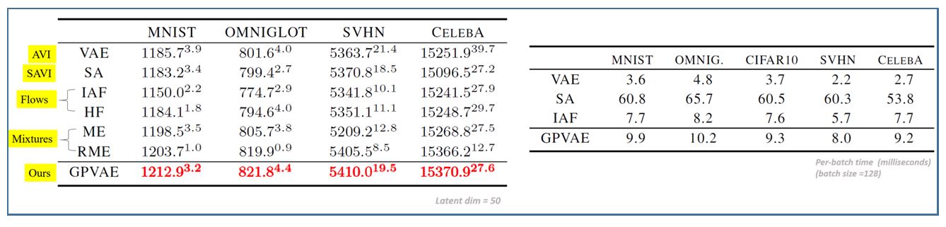
Table 1. (Left) Test log-likelihood scores and (Right) per-batch inference times (milliseconds).
Uncertainty vs. Approximation Difficulty
In our GPVAE model, the posterior variances of the error functions, that is,  , indicate uncertainty or goodness of amortized approximation. In Figure. 3, for the MNIST dataset with 2D latents, we show some examples with different uncertainty scores, from low to high. It shows that low uncertainty corresponds to easy approximation (visually large overlap between the true and approximate posteriors; and also showing better reconstruction), whereas high uncertainty means more difficult approximation (posteriors considerably mismatch with worse reconstruction).

Figure 3. Uncertainty vs. posterior approximation difficulty. After the GPVAE model is trained on MNIST with 2D latent space, we evaluate the uncertainty  and depict six different instances
  in the order of increasing uncertainty values. (Top panel) The true posterior
  (contour plots) and the base encoder
  (red dots) superimposed (in log scale). (Bottom panel) Original inputs (left) and reconstructed images (right). For the cases with lower uncertainty, the true posteriors are more Gaussian-like. On the other hand, the higher uncertainty cases have highly non-Gaussian true posteriors with multiple modes.
Conclusion
In this blog we presented our recent work on Gaussian process inference error modeling for VAE. Our approach significantly reduces the posterior approximation error of the amortized inference in VAE, while being computationally efficient. Our Bayesian treatment that regards the discrepancy in posterior approximation as a random noise process, leads to improvements in the accuracy of inference within the fast amortized inference framework. It also offers the ability to quantify the uncertainty (variance of stochastic noise) in variational inference, intuitively interpreted as inherent difficulty in posterior approximation.
As future work we can carry out more extensive experiments, e.g., deeper network architectures, hierarchical models, or larger/structured latent spaces. In particular, the latest denoising diffusive generative models [9,10] form a highly sequential sparse structure in the latent space, and it is very interesting future work to investigate how the proposed inference error modeling can be applied to such a structured inference model. In the current work we mainly aimed to focus on proving our concept, and this was done with popular VAE frameworks on benchmark datasets that we used. Another important future study not included in this paper is the rigorous analysis of the impact of the series of approximations that we used in our model.
Lastly, there are numerous interesting application areas for which the proposed GPVAE inference algorithm can be beneficial. They range from more realistic data synthesis including virtual avatars for video teleconferencing and image editing, to more accurate factor analysis in highly structured data such as videos, natural language texts, audio/speech signals, and also data with complex interactions including biological sequences, molecular graphs, and general 3D shapes.
Link to the paper
References
[1] M. Kim, Gaussian Process Modeling of Approximate Inference Errors for Variational Autoencoders, In Computer Vision and Pattern Recognition, 2022.
[2] C. E. Rasmussen and C. K. I. Williams, Gaussian Processes for Machine Learning. The MIT Press, 2006.
[3] A. G. Wilson, Z. Hu, R. Salakhutdinov, and E. P. Xing, Deep kernel learning, AI and Statistics, 2016.
[4] M. Kim and V. Pavlovic, Recursive Inference for Variational Autoencoders, In Advances in Neural Information Processing Systems, 2020.
[5] D. P. Kingma and M. Welling. Auto-encoding variational Bayes, In International Conference on Learning Representations, 2014.
[6] D.J. Rezende, S. Mohamed, and D. Wierstra. Stochastic backpropagation and approximate inference in deep generative models, In International Conference on Machine Learning, 2014.
[7] Y. Kim, S. Wiseman, A. C. Millter, D. Sontag, and A. M. Rush. Semi-amortized variational autoencoders, In International Conference on Machine Learning, 2018.
[8] D. P. Kingma, T. Salimans, R. Jozefowicz, X. Chen, I. Sutskever, and M. Welling. Improving variational inference with inverse autoregressive flow, In Advances in Neural Information Processing Systems, 2016.
[9] Y. Song and S. Ermon, Generative modeling by estimating gradients of the data distribution. In Advances in Neural Information Processing Systems, 2019.
[10] J. Ho, A. Jain, and P. Abbeel, Denoising Diffusion Probabilistic Models, In Advances in Neural Information Processing Systems, 2020.