AI
Fast and Accurate Inference in Variational Autoencoders
Variational Autoencoders (VAE) [2,3] and Generative Adversarial Networks (GAN) [4] are the most popular deep generative models for high dimensional data (e.g., images). Although both models employ similar neural net architectures for data synthesis z->x (from latent variables z to a data instance/image x), VAE has an inference model x->z, which GAN lacks, and this endows VAE with the unique capability of interpreting and directly controlling the latent variables that correspond to underlying hidden factors in data generation. The vanilla VAE performs the inference (x->z) by a single feed-forward pass through a neural network (aka encoder network), which is trained by the maximum likelihood learning criterion. This, referred to as amortized inference, enables fast inference, however, it comes at the cost of accuracy degradation oftentimes, known as the amortization error. Recently several attempts were made to address this accuracy issue. In this blog, we present our latest work Recursive Mixture Inference [1] that yields more accurate inference than the state-of-the-arts, while being as fast as the vanilla VAE.
VAE and (Stochastic) Variational Inference
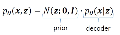
In the probabilistic view, VAE models a joint distribution that can be decomposed into the Gaussian prior and the conditional decoding process which is modeled by a (deep) neural network with parameters \[θ\]
We are particularly interested in posterior inference, i.e., the distribution of the latent variables z given the observed (evidence) x, which is required during both training and test time. And the posterior is defined by the Bayes rule:
\[p_{\theta}({\bf x},{\bf z}) = \frac{N({\bf z};\mathbf{0},{{\bf \it I}})\cdot p_{\theta}({\bf x}|{\bf z})}{\int_{}N({\bf z};\mathbf{0},{{\bf \it I}})\cdot p_{\theta}({\bf x}|{\bf z})d{\bf z}}\]
Unfortunately, this posterior distribution cannot be computed exactly due to the intractable integration in the denominator. There exist several approximate inference methods that lead to tractable approximation of the true posterior, among which VAE adopts the variational inference (VI), as is guessed from its name.
Often referred to as SVI (stochastic VI), the basic idea is to approximate the true posterior by a tractable distribution such as Gaussian \[q_{\lambda}\left({\bf z}\right)=N\left({\bf z};{\bf{\mu}},\mathbf{\Sigma}\right)\], parameterized by \[\ {\bf{\lambda}}=({\bf{\mu}},\mathbf{\Sigma})\]. The posterior inference in SVI amounts to finding the Gaussian that is closest to the true posterior, that is,
\[\min_{\lambda} KL(q\lambda({\bf z})||p_{\theta}({\bf z}|{\bf x}))\]
And it can be shown that the \[KL\] divergence, the error between true and approximate posteriors, equals (up to constant) what is called ELBO (evidence lower bound) function \[L\left({\bf {\lambda}},{\bf{\theta}};{\bf{x}}\right)\] with the opposite sign,

Then, minimizing the \[KL\], equivalently maximizing the ELBO, can be done by stochastic gradient descent (SGD), as illustrated in Fig. 1. However, the critical drawback of SVI is that the ELBO objective is specific to the instance x, and when a new instance x comes in, the SGD optimization has to be performed from the outset. That is, SVI is computationally very expensive. See Fig. 1.
\[ {{\lambda}_{\color{red}x}^\ast=argmax_{\lambda}{\ L\left({\lambda},{\theta};{\color{red}x}\right)}}\]
\[ {{\lambda}_{\color{blue}x\color{blue}\prime}^\ast=argmax_{\lambda}{\ L\left({\lambda},{\theta};{\color{blue}x\color{blue}\prime}\right)}}\]
Fig. 1. (Animated GIFs) For two different instances x and x’, their ELBO objectives are different since the true posteriors, shown as contours, are different. This means that one has to solve the SVI optimization independently for each one, from the outset.
Amortized Inference
In the original VAE papers [2,3], SVI’s computational issue was addressed by the so-called amortized inference (AVI). The optimal solution of the SVI optimization problem can be seen as a function of \[\it \bf x\], i.e., \[{\bf {\lambda}}^\ast\left({\bf {x}}\right)=argmax_\lambda{\ L\left({\bf {\lambda}},{\bf {\theta}};{\bf {x}}\right)}\], and we can train a neural network to mimic this function \[{\bf {\lambda}}^\ast\left({\bf{x}}\right)\approx{\bf{\lambda}}({\bf{x}};{\bf{\phi}})\], which is reasonable due to the principle of the universal function approximator. This is called amortized inference (Fig. 2), a remarkable idea that replaces the time-consuming SVI optimization at inference time by a single feed-forward pass through a neural network (called the inference or encoder network).
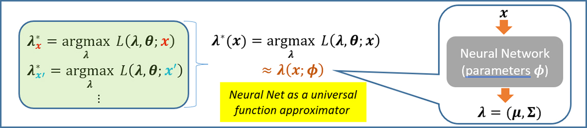
Fig. 2. Amortized inference. It replaces the SVI optimization problem by a single feed-forward pass through a neural network called the inference/encoder network \[\bf {\lambda}({x};{\phi})\], with parameters \[\bf {\phi}\].
However, this computational advantage does not come without a cost; AVI is fast, but less accurate than SVI due to the neural net function approximation error, also known as the amortization gap. See Fig. 3.
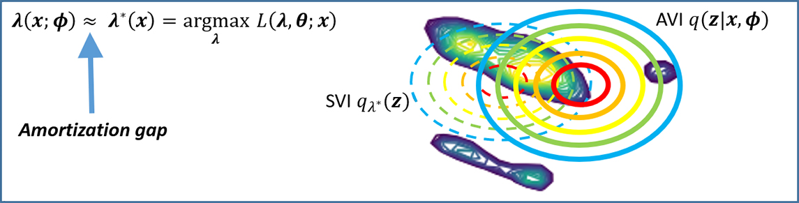
Fig. 3. Amortization gap makes AVI less accurate than SVI.
Semi-Amortized VI
There have been considerable attempts to reduce the amortization gap, and the semi-amortized VI (SAVI for short) is one successful line of approaches [5]. The core idea is to take the benefits of the amortized inference and SVI’s gradient-based update, specifically by taking a few SVI gradient steps starting from the posterior approximation obtained by AVI. That is, SAVI can be seen as a warm-start SVI with the initial iterate \[ q_{\lambda}\left({\bf{z}}\right)\], where \[\bf {\lambda}=\left({\mu},{\Sigma}\right)={\lambda}({x};{\phi})\] is the output of the amortized encoder network. See Fig. 4 for illustration.

Fig. 4. (Animated GIF) Semi-Amortized VI (SAVI) refines the posterior output from the encoder network by a few extra SVI gradient steps.
The SVI gradients steps (usually 1~8 steps taken) refines potentially less accurate AVI posterior, and reduces the amortization gap. Note that the SAVI training still aims to learn the encoder network parameters \mathbit{\phi}, and this is done by doing backpropagation from the (ELBO) objective function defined with the final refined posterior of SAVI, down to \mathbit{\phi}. This means that we need to take derivatives of the SVI gradients, that is, high-order derivatives (e.g., Hessians). Although there exist several approximation schemes (e.g., finite difference methods) to circumvent Hessian-vector computation, SAVI inherently suffers from the computationally overhead.
Our Approach: Recursive Mixture Inference
To have an inference model that is accurate and fast (faster than SAVI), we propose a novel recursive mixture inference. The idea is to incrementally augment the amortized encoders, one at a time, by forming a mixture of encoder networks. The concept is best understood by seeing the diagram in Fig. 5. Initially, the mixture \[ Q({\bf{z}}|{\bf{x}})\]is composed of a single encoder network \[ \color{blue} {q({\bf{z}}|{\bf{x}},{\bf{\phi}})}\] which can be the amortized encoder from the vanilla VAE (shown as the elliptical contour in the left panel in Fig. 5). This current posterior may be not so accurate, exhibiting considerable mismatch with the true posterior (the green-colored contour). We hence add another encoder \[ \color{red} {q\prime({\bf{z}}|{\bf{x}},{\bf{\phi}}\prime)}\], with a small mixing proportion \epsilon, whose support occupies regions that were not covered by the current posterior (middle panel in Fig. 5). Note that we find a new amortized encoder (with the neural net parameters \[\color{red} {{\phi}\prime}\]) instead of performing any gradient-based refinement as SAVI does, which removes SAVI’s aforementioned computational issue.
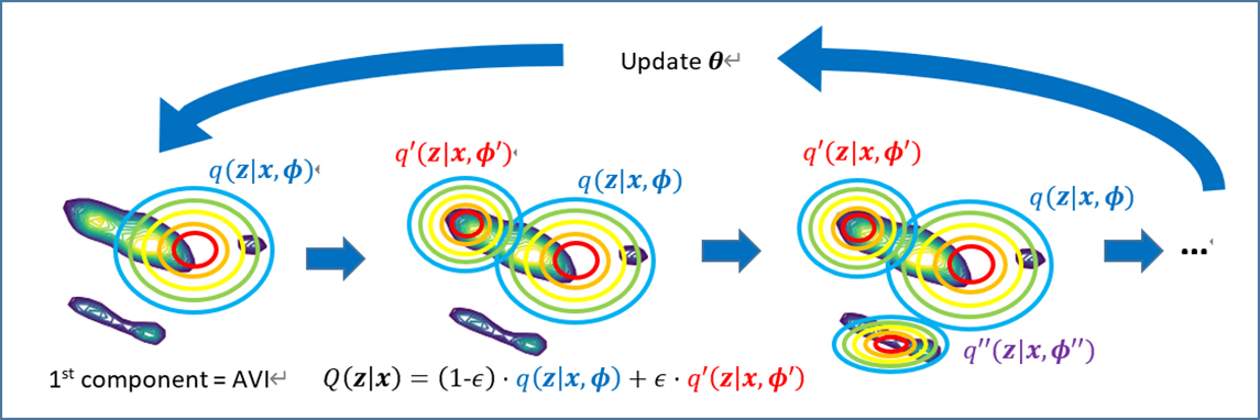
Fig. 5. Concept diagram for training of our recursive mixture inference model.
The key question is how to select (i.e., learn) the new component \[\color{red} { q\prime({\bf{z}}|{\bf{x}},{\bf{\phi}}\prime)}\], and we consider two selection criteria: 1) the new component \[\color{red} {q\prime}\], in conjunction with the current mixture, has to reduce the posterior approximation error (the error between the true and approximate posteriors), and 2) \[\color{red} {q\prime}\] needs to be different from the current mixture to remove redundancy and increase diversity of the new posterior. The latter criterion is beneficial to avoid the component collapsing, the well-known issue often observed in the conventional (end-to-end or EM-based) mixture learning. To meet the criteria, we derive a novel learning objective using the functional gradient (boosting) principle [6,7], which is summarized in Fig. 6. The first term is the ELBO of the new component that directly aims for the first criterion, while the second term, the KL divergence between the new component and current mixture, is tied to the second criterion. The interested readers are encouraged to refer to our paper [1] for the full derivation.
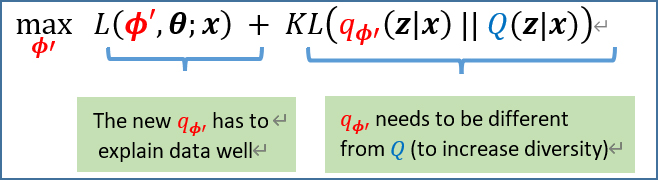
Fig. 6. Our selection criteria for a new mixture component as a learning problem.
This procedure continues recursively to add the third, fourth components, and so on. When we reach the predefined mixture order (usually from 2 to 5), we update the VAE model parameters \[\theta\] (the decoder parameters), and also iteratively refine the parameters of the mixture components. We repeat these training iterations until convergence, and as a result we end up with the mixture of amortized encoder networks as our posterior inference model.
The main benefit of our approach, compared to SAVI, is fast and accurate inference. Our inference model does not involve computationally expensive gradient steps at inference time, and the input instances just need to pass through the multiple neural net encoders (components of the mixture), hence fast. And it can be even faster if we implement the encoder feed-forwards to be done in parallel (although we have not done it yet in our current implementation and experiments).
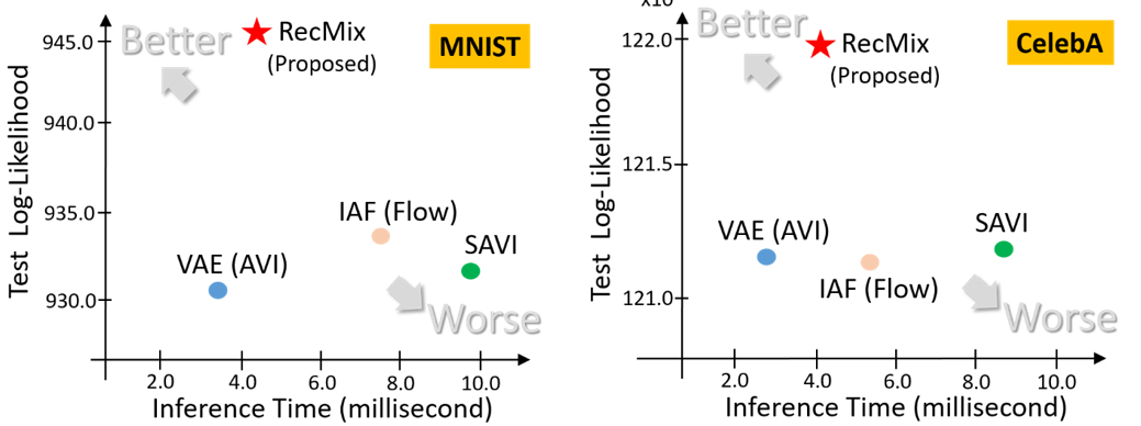
Fig. 7. Test log-likelihood scores and inference times of competing approaches on MNIST and CelebA. In each XY plane, the points at upper-left corner indicate preferable approaches, while those at the lower-right corner are less preferable.
Experimental Results
We measure the generalization performance and inference time of the proposed method (dubbed RecMix) on several benchmark datasets, where we show results only on the MNIST and CelebA datasets (please refer to [1] for full experimental results). Our approach is contrasted with the vanilla VAE (AVI), SAVI [5], and the flow-based model IAF [8] that has rich representational capacity. The results are visualized in Fig. 7. Our RecMix method achieves the highest test likelihood scores (even better than the complex flow-based encoder model), with inference time comparable to VAE (AVI) and significantly lower than SAVI.
Conclusion
In this blog we presented a novel mixture inference model to improve traditional amortized inference in VAEs. The recursive estimation strategy makes the approach both effective in increasing the accuracy of inference and computationally efficient, compared to state-of-the-art semi-amortized inference methods. Our approach yields higher generalization performance than the state-of-the-arts on several benchmark datasets, but remains as computationally efficient as the conventional VAE inference. Our model currently requires users to supply the mixture order as an input to the algorithm. In our future work, we will investigate principled ways of selecting the mixture order (i.e., model augmentation stopping criteria).
There are numerous interesting application problems for which the proposed recursive VAE inference algorithm can be beneficial. They include multi/cross-modal structured data such as videos, natural language sentences, audio/speech signals, and also data with complex interactions including biological sequences, molecular graphs, and 3D shapes. These exciting application areas will be discussed in our upcoming blog post.
Publication
https://papers.nips.cc/paper/2020/file/e3844e186e6eb8736e9f53c0c5889527-Paper.pdf
Reference
[1] M. Kim and V. Pavlovic, Recursive Inference for Variational Autoencoders, In Advances in Neural Information Processing Systems, 2020.
[2] D. P. Kingma and M. Welling. Auto-encoding variational Bayes, In International Conference on Learning Representations, 2014.
[3] D.J. Rezende, S. Mohamed, and D. Wierstra. Stochastic backpropagation and approximate inference in deep generative models, In International Conference on Machine Learning, 2014.
[4] I. Goodfellow, J. Pouget-Abadie, M. Mirza, B. Xu, D. Warde-Farley, S. Ozair, A. Courville, and Y. Bengio. Generative Adversarial Networks, In Advances in Neural Information Processing Systems, 2014.
[5] Y. Kim, S. Wiseman, A. C. Millter, D. Sontag, and A. M. Rush. Semi-amortized variational autoencoders, In International Conference on Machine Learning, 2018.
[6] J. Friedman. Greedy function approximation: A gradient boosting machine, 1999. Technical Report, Dept. of Statistics, Stanford University.
[7] L. Mason, J. Baxter, P. Bartlett, and M. Frean. Functional gradient techniques for combining hypotheses. In Advances in Large Margin Classifiers, MIT Press, 1999.
[8] D. P. Kingma, T. Salimans, R. Jozefowicz, X. Chen, I. Sutskever, and M. Welling. Improving variational inference with inverse autoregressive flow, In Advances in Neural Information Processing Systems, 2016.